Part 4: Deterministic Networks for Physical AI

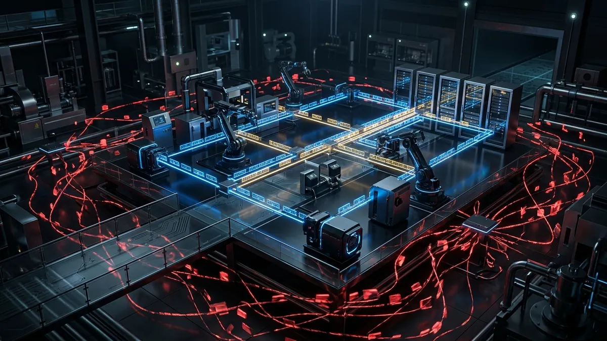
When streaming a 4K video over a conventional best-effort network, the application can tolerate variations in network delivery. The transport layer relies on buffering, reliable byte-stream delivery, and error concealment to smooth out the bumps. For video, arriving slightly late can still be useful.

However, if a multi-axis industrial robot is waiting for position telemetry in a hard real-time control loop, it does not have the luxury of buffering. For a control loop, arriving late renders the information useless.

This temporal strictness exposes a fundamental limitation of best-effort networking: optimizing for average throughput and utilization does not automatically provide bounded latency and jitter.

The Temporal Problem

For Physical AI, a network packet has two dimensions of correctness: what it contains and when it arrives.

Traditional best-effort networking generally treats the second as a statistical property rather than an explicitly bounded one. But consider the reality of a robotic control loop:

flowchart TD
    T0["t0: Sensor measures robot position"] --> Delayed["Packet delayed by network congestion"]
    Delayed --> T1["t1: Robot physically moves"]
    T1 --> Wrong["Controller receives t0 position"]

When the controller finally receives the delayed packet, the packet isn’t corrupted. Rather, it contains correct historical data arriving at the wrong time. The packet itself is not incorrect. Its meaning has expired. The delayed packet is no longer just late; it is dangerously incorrect because the physical state of the world has already changed.

Physical AI does not require impossible mathematical guarantees of zero latency. It requires predictable, bounded timing behavior.

Why Best-Effort Networking Isn’t Enough

In traditional Ethernet and best-effort IP networks, switches forward packets as quickly as possible. If multiple devices transmit at the exact same moment, the packets enter a queue. This contention creates jitter (variance in latency) and expands the tail latency of the network.

In many cloud workloads, a few milliseconds of additional queueing delay may have little user-visible impact. But in a robotic control loop with a total budget of 10 milliseconds, that same delay can completely invalidate the timing assumptions of the control loop.

Enter Time-Sensitive Networking (TSN)

To solve the temporal synchronization problem, industrial networking is turning to Time-Sensitive Networking (TSN)—a family of IEEE standards that upgrade standard Ethernet from a best-effort delivery system into a deterministic, time-aware fabric.

TSN is not a replacement for Ethernet or IP; rather, several TSN mechanisms work together to provide bounded behavior at the network layer. Four of the most critical mechanisms are:

1. Hardware-Assisted Clock Synchronization: PTP (IEEE 1588), often combined with IEEE 802.1AS in TSN profiles, can synchronize participating devices to sub-microsecond accuracy under appropriate hardware and network conditions.
2. Time-Aware Traffic Scheduling: Instead of relying entirely on conventional queuing, the network operates on a strict schedule. Critical traffic can be assigned scheduled transmission opportunities on the link at pre-calculated intervals.
3. Frame Preemption: If a large, non-critical frame is being transmitted when a critical express frame needs the link, frame preemption (IEEE 802.1Qbu/802.3br) allows the critical frame to interrupt. The preempted frame is fragmented into smaller pieces and resumed afterward.
4. Reliability and Redundancy (FRER): Physical AI requires timely delivery and resilience to link failures. Frame Replication and Elimination for Reliability allows redundant paths to carry copies of critical frames, while the receiver eliminates duplicate frames.

The goal of deterministic networking is therefore not to make every packet fast. It is to make critical traffic predictably fast.

Architectural Trade-offs

Characteristic	Best-Effort Ethernet/IP	Time-Sensitive Networking (TSN)
Timing Model	Statistical / best-effort	Bounded and engineered
Latency	Variable	Designed around bounded latency
Jitter	Can vary with congestion	Can be tightly bounded
Clock Sync	Typically application/system dependent	Network-wide (PTP / IEEE 802.1AS)
Traffic Handling	Conventional queuing	Shaping, scheduling, preemption
Configuration	Relatively simple	More complex, topology-aware

The trade-off for determinism is configuration complexity. Adding new critical traffic or changing the topology can require the schedules and stream configuration to be recomputed or revalidated, increasing operational overhead.

Determinism Is a System Property

Crucially, deterministic networking does not exist in isolation.

flowchart LR
    S["Sensor"] --> NIC["TSN NIC"]
    NIC --> SW["TSN Switch"]
    SW --> CTRL["AI Control"]
    
    subgraph Budget["Deterministic timing budget"]
        direction LR
        NIC
        SW
        CTRL
    end
    
    CTRL --> ACT["Actuator"]

The entire path—from the physical sensor, through the NIC, across the switches, into the AI controller, through the software stack, and back out to the actuator—must respect the timing budget. You cannot build a network engineered for 100 µs-class jitter and then spend 8 milliseconds waiting in an unoptimized software queue on the host OS.

Determinism is an end-to-end system property.

Conclusion

Network engineering in the era of Physical AI must evolve from a best-effort transport into an engineered, time-aware fabric with explicit latency, jitter, synchronization, and reliability objectives. Physical AI doesn’t just need more bandwidth; it needs control over time.

---

What’s Next?

We have solved how to ingest reality (Part 2), where to compute it (Part 3), and how to engineer its timely delivery across the network (Part 4).

But how do you retain enough physical experience to continuously improve the World Model without storing everything the sensors ever observed?

In Part 5, we will tackle the final bottleneck: The Memory Wall — Storing Reality for World Models.