Part 3: The Compute Split - Edge vs Cloud in Physical AI

“We cannot defeat the speed of light. Therefore, the intelligence must live where the action happens.”

In Part 2, we identified the Data Ingestion Wall—the fundamental systems bottleneck created by continuous, high-bandwidth reality streams pouring out of physical AI sensors.

To overcome this, we must accept a harsh reality about physics and networking: the cloud is too far away for the hard real-time control loop.

When dealing with large language models, a delay of 200 milliseconds to receive a generated token from a remote server is considered an excellent user experience. However, if a warehouse robot traveling at 3 meters per second waits 200 milliseconds for a cloud server to tell it whether an object is a shadow or a human, the robot will have traveled over half a meter blind.

This brings us to the most defining architectural paradigm of Physical AI: The Compute Split.

The Compute Split

Physical AI cannot be architected around a single centralized intelligence. A practical architecture separates intelligence by time horizon rather than treating the model as a single monolithic system.

flowchart TD
    subgraph Edge["HARD REAL-TIME DOMAIN (Edge)"]
        direction TB
        S["Sensors"] --> F["Fusion"]
        F --> LM["Local Model"]
        LM --> A["Actuators"]
    end
    
    subgraph Cloud["CLOUD DOMAIN"]
        direction TB
        Sim["Simulation"] --> T["Training"]
        T --> E["Evaluation"]
    end
    
    F -.->|"Telemetry"| Sim
    E -.->|"Model/Policy Updates"| LM

The Latency Budget

Every physical action taken by an autonomous agent is governed by a strict, unforgiving timeline known as the Latency Budget.

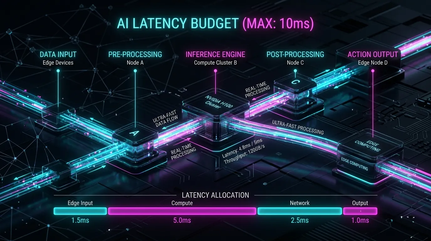An illustration of an AI latency budget showing real-time processing constraints.

Consider an illustrative high-speed robotic system with a 10 ms end-to-end budget:

Phase	Allotted Time	Primary Function	Hardware Target
Capture & Sync	1.5 ms	Acquire frame, hardware timestamping, align clock domain.	ISP / Edge NIC
Perception	3.0 ms	Identify object velocity, trajectory, and spatial boundaries.	Edge NPU / GPU
Local Prediction / Policy	4.5 ms	Predict future physics state; compute grip force and safety margins.	High-Perf Edge Accelerator
Actuation	1.0 ms	Transmit command to physical motor controllers.	Deterministic Network
Total Latency	10.0 ms	End-to-End Sense-Think-Act Loop	Physical Edge System

If we attempt to perform the “World Model Inference” phase in a centralized cloud data center located 500 miles away, we hit a physical wall. A 500-mile separation has an approximate theoretical propagation floor in fiber of roughly 8 ms round trip. Real networks add routing, switching, serialization, and queuing overhead, making a 10–15 ms RTT entirely plausible under favorable conditions.

The latency budget is blown before the neural network even begins to compute.

Why Reaction Must Stay at the Edge

Because we cannot defeat the speed of light over fiber optics, the immediate, reactive intelligence must be pushed to the very edge of the network—often directly onto the robot or the factory floor server.

What runs at the edge?

• Sensor Fusion & Preprocessing: Compressing and discarding irrelevant data (as discussed in Part 2).
• Local Models: Quantized, highly-optimized subsets, learned policies, or classical controllers that specialize in immediate physics predictions.
• Safety Guardrails: Hardcoded or lightweight safety mechanisms designed to keep the system within defined operating limits even if the primary AI fails.

The challenge at the edge is not intelligence, but constraints. A mobile robot has limited space, battery power, and cooling capacity. Edge compute relies heavily on highly efficient NPUs and tight memory integration.

The edge reacts. The cloud learns.

Why Learning Moves to the Cloud

If the edge handles the reaction, the cloud handles the evolution.

A World Model contains a generalized understanding of the physics of countless environments. This larger intelligence can leverage elastic compute, storage, and accelerator capacity in centralized infrastructure.

What belongs in the cloud?

• Global State Aggregation: Building a digital twin of an entire fleet or facility across millions of hours of operation.
• Continuous Learning: Retraining foundational models based on new edge data.
• The “Simulation Engine”: When an edge device encounters a failure (e.g., a robot slips on a new type of oil), that specific telemetry is uploaded. The cloud recreates that exact physical scenario in a virtual simulator, generates thousands of synthetic permutations of the event, and trains the model on how to handle it perfectly.

We call this “Re-simulating Reality.”

The Synchronization Problem

If intelligence is split based on time horizons, how does the system stay aligned?

Time Horizon	Responsibility	Location
µs – ms	Motor control & safety	Device / Edge
ms – 100 ms	Perception & reactive inference	Edge
Seconds – minutes	Planning & coordination	Edge / Local / Cloud
Hours – days	Fleet optimization	Cloud
Days – weeks	Training & simulation	Cloud

The split is therefore not simply about where compute is cheaper. It is about where a decision can be made within its required time and reliability envelope.

This is the frontier of AI systems engineering: Model Synchronization over Low-Bandwidth Links.

One possible direction is to move away from monolithic model replacement toward smaller, targeted model updates. When the cloud simulator discovers a new physics rule, it doesn’t necessarily send the entire model to the edge. Instead, it relies on model deltas, adapters, distillation, or policy patches to transmit highly compressed, targeted updates to the edge models.

The Tail-Latency Problem: What the Cloud Cannot Guarantee

A cloud service cannot provide a hard guarantee for a physical control loop merely by having a low average latency.

What matters is the tail of the latency distribution. p50 latency can hide the rare delays that are unacceptable to a physical control loop. Depending on the system’s safety requirements, engineers may need to reason about p99, p99.9, p99.99, or explicit worst-case bounds. Jitter, congestion, route changes, and packet loss can all expand that tail. A system operating a physical machine cares about the worst acceptable execution window, not merely average latency.

Architectural Summary

Characteristic	Edge Inference	Cloud Intelligence
Primary Goal	Instantaneous reaction & safety	Continuous evolution & simulation
Model Profile	Task-specific, optimized, quantized	Larger, generalized, continuously evolving
Execution	Deterministic / bounded	Asynchronous / elastic
Data Flow	Synchronized reality streams (Ingress)	Model deltas & adapters (Egress)

---

What’s Next?

We know where the compute must live based on the time horizon of the decision. But how do we engineer the network so that critical data arrives within a bounded latency and jitter budget, even when the network is congested?

In Part 4, we will explore why conventional best-effort IP networking is insufficient for hard real-time Physical AI, and how Deterministic Networks (TSN) are changing the fabric of industrial connectivity.